Introduction
The fundamental relationship among the three important electrical quantities current, voltage, and resistance was discovered by Georg Simon Ohm. The relationship and the unit of electrical resistance were both named for him to commemorate this contribution to physics. One statement of Ohm’s Law is that the current through a resistor is proportional to the voltage across the resistor and inversely proportional to the resistance. In this experiment we will see if Ohm’s Law is applicable by generating experimental data using a PhET Simulation:
https://phet.colorado.edu/en/simulation/legacy/ohms-law
Current and voltage can be difficult to understand, because they cannot be observed directly. To clarify these terms, some people make the comparison between electrical circuits and water flowing in pipes. Here is a chart of the three electrical units we will study in this experiment.
Electrical Quantity |
Description |
Unit |
Water Analogy |
Voltage or Potential Difference |
A measure of the Energy difference per unit charge between two points in a circuit. |
Volt (V) |
Water Pressure |
Current |
A measure of the flow of charge in a circuit. |
Ampere (A) |
Amount of water flowing |
Resistance |
A measure of how difficult it is for current to flow in a circuit. |
Ohm (\( \Omega \)) |
A measure of how difficult it is for water to flow through a pipe. |

Figure 1
Objectives
- Determine the mathematical relationship between current, potential difference, and resistance in a simple circuit.
- Examine the potential vs. current behavior of a resistor and current vs. resistance for a fixed potential.
Materials
- Computer
- PhET Simulation - Ohm's Law
- Logger Pro, from Vernier Software
Preliminary Setup and Questions
|
| ||
- With the Resistance slider set at \( 550 \Omega \) (the default), move the Voltage slider, observing what happens to the current.
- If the voltage doubles, what happens to the current?
- If the voltage doubles, so does the current. They seem to be linked.
- What type of relationship do you believe exists between voltage and current?
- I believe voltage and current are directly proportional.
- If the voltage doubles, what happens to the current?
- With the Voltage slider set at \( 4.5 \text{V} \) (the default), move the Resistance slider, observing what happens to the current.
- If the resistance doubles, what happens to the current?
- If the resistance doubles, the current is divided by two. They also seem to be linked.
- What type of relationship do you believe exists between current and resistance?
- I believe current and resistance are inversely proportional.
- If the resistance doubles, what happens to the current?
Procedure
- Set the Resistance slider to \( 300 \Omega \). Use the Voltage slider to adjust the potential (aka voltage) to the values in Data Table 1, also recording the resulting electric currents.
Data Table 1
Resistance: \( R = 300 \Omega \)
Resistance: \( R = 300 \Omega \)
Current (mA) |
Potential (V) |
Current (mA) |
Potential (V) |
5.0 |
1.5 |
20.0 |
6.0 |
10.0 |
3.0 |
25.0 |
7.5 |
15.0 |
4.5 |
30.0 |
9.0 |
Slope of graph = \( 0.3 \frac{ \text{V} }{ \text{mA} } \)
Slope times 1000 = \( 300 \Omega \)
% Error of Slope times 1000 with \( R \) = \( 0 \% \)
Slope times 1000 = \( 300 \Omega \)
% Error of Slope times 1000 with \( R \) = \( 0 \% \)
Switch to Logger Pro. Enter your data from Data Table 1 into Data Set 1. Perform a "linear fit" on the data. Record the slope of the graph below Data Table 1.
Calculate the resistance value by taking the slope of the graph and multiplying by 1000. Compare this new value with the value of the resistance set in the simulation by calculating a % error.
Calculate the resistance value by taking the slope of the graph and multiplying by 1000. Compare this new value with the value of the resistance set in the simulation by calculating a % error.
- Switch back to the PhET Simulation.
- Set the Resistance slider to \( 600 \Omega \). Use the Voltage slider to adjust the potential (aka voltage) to the values in Data Table 2, also recording the resulting electric currents.
Data Table 2
Resistance \( R = 600 \Omega \)
Resistance \( R = 600 \Omega \)
Current (mA) |
Potential (V) |
Current (mA) |
Potential (V) |
2.5 |
1.5 |
10.0 |
6.0 |
5.0 |
3.0 |
12.5 |
7.5 |
7.5 |
4.5 |
15.0 |
9.0 |
Slope of graph = \( 0.6 \frac{ \text{V} }{ \text{mA} } \)
Slope times 1000 = \( 600 \Omega \)
% Error of Slope times 1000 with \( R \) = \( 0 \% \)
Slope times 1000 = \( 600 \Omega \)
% Error of Slope times 1000 with \( R \) = \( 0 \% \)
Switch to Logger Pro. Enter your data from Data Table 2 into Data Set 2. Perform a "linear fit" on the data. Record the slope of the graph below Data Table 2.
Calculate the resistance value by taking the slope of the graph and multiplying by 1000. Compare this new value with the value of the resistance set in the simulation by calculating a % error.
Paste the resulting graphs for both data sets with fits showing:
Calculate the resistance value by taking the slope of the graph and multiplying by 1000. Compare this new value with the value of the resistance set in the simulation by calculating a % error.
Paste the resulting graphs for both data sets with fits showing:
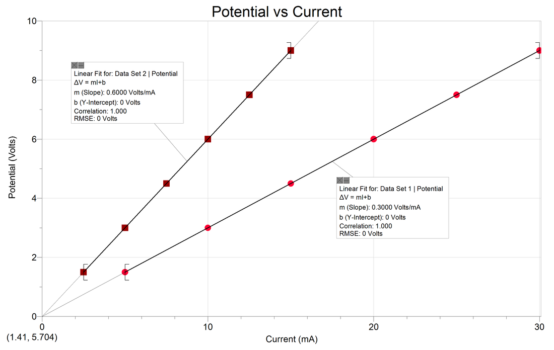
Does a linear function work well with both data sets of \( V \) vs \( I \) data? Yes.
- Switch back to the PhET simulation.
- Return the Voltage Slider to \( 4.5 \text{V} \). Now we will use the Resistance slider to adjust the resistance to the values in Data Table 3, also recording the resulting electric currents.
Data Table 3
Electric Potential, or Voltage: \( V = 4.5 \text{V} \)
Electric Potential, or Voltage: \( V = 4.5 \text{V} \)
R (\( \Omega \)) |
Current (mA) |
R (\( \Omega \)) |
Current (mA) |
100 |
45.0 |
600 |
7.5 |
200 |
22.5 |
700 |
6.4 |
300 |
15.0 |
800 |
5.6 |
400 |
11.3 |
900 |
5.0 |
500 |
9.0 |
1000 |
4.5 |
Inverse Fit Constant of graph of \( I \) vs \( R \) = \( 4500 \Omega \text{mA} \)
Inverse Fit Constant divided by 1000 = \( 4.5 \text{V} \)
% Error of Fit Constant Divided by 1000 with \( V \) = \( 0 \% \)
Inverse Fit Constant divided by 1000 = \( 4.5 \text{V} \)
% Error of Fit Constant Divided by 1000 with \( V \) = \( 0 \% \)
Switch to Logger Pro. Go to Page 2 on the display. Enter your data from Data Table 3 into Data Set 3. Using "Curve Fit," perform an “Inverse” fit on the data. Record the Inverse Fit Constant below Data Table 3.
Calculate the voltage value by taking the Inverse Fit Constant and dividing by 1000. Compare this new value with the value of the voltage set in the simulation by calculating a % error.
Paste the resulting graph for Data Set 3 with the fit showing:
Calculate the voltage value by taking the Inverse Fit Constant and dividing by 1000. Compare this new value with the value of the voltage set in the simulation by calculating a % error.
Paste the resulting graph for Data Set 3 with the fit showing:

Does an inverse function provide a good fit to your data? Yes.
Analysis
- Does the experimental data confirm that the electric current in a resistor is directly proportional to the electric potential provided by the batteries?
- Yes, it is confirmed. When graphed, we could easily see that there is a direct relationship between current and electric potential, thanks to the constant slope.
- Does the experimental data confirm that the electric current is inversely proportional to the resistance for a fixed electric potential?
- Yes, it is confirmed. When graphed, we could easily see that there is an inverse relationship between current and resistance, thanks to the exponential decay we observe in the slope.
Conclusion
- Write a conclusion that summarizes the results of this experiment.
- After conducting this experiment, I feel I understand Ohm's Law quite clearly, and how current, resistance, and voltage (aka electric potential) are related.
This relationship comes in a few forms, depending on which value we're solving for:- Current: \( I = \frac{ V }{ R } \)
- Voltage: \( V = I \cdot R \)
- Resistance: \( R = \frac{ V }{ I } \)
- After conducting this experiment, I feel I understand Ohm's Law quite clearly, and how current, resistance, and voltage (aka electric potential) are related.
